Difference between revisions of "Free Fall (determination of the standard gravity)"
(→Description of the Experiment: Adicionada caixa de ligações) |
|||
| Line 1: | Line 1: | ||
=Description of the Experiment= | =Description of the Experiment= | ||
| − | This experiment | + | This experiment allows to determine the standard gravity acceleration, <i>g </i>. |
<div class="toccolours mw-collapsible mw-collapsed" style="width:300px"> | <div class="toccolours mw-collapsible mw-collapsed" style="width:300px"> | ||
| Line 15: | Line 15: | ||
=Experimental Apparatus= | =Experimental Apparatus= | ||
| − | This apparatus | + | This apparatus consist in a projectile launcher (with an electromagnet) that vertically ejects a ping-pong ball from the base. |
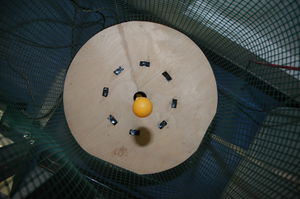
[[File:Gravidade-montagem.jpg|thumb|alt=Esperimental setup|Setup]] | [[File:Gravidade-montagem.jpg|thumb|alt=Esperimental setup|Setup]] | ||
| − | The ping-pong ball is launched with a kinetic energy selected by the user (energy applied to the electromagnet) and | + | The ping-pong ball is launched with a kinetic energy from the base selected by the user (energy applied to the electromagnet) and executes the typicall parabola trajectory, falling subsequently on the base. The height (vertical coordinate) is measured and recorded with an ultrasound sonar, strategically placed above the experiment, measuring the distance between itself and the ball. With the resulting data it is possible to determine <i>g</i>. The ball is sometimes launched with a small horizontal component, but this does not affect measurements (why?). |
| − | Since the height is measured by | + | Since the height is measured by ultrasounds, the actual time between samples varies from the one provided by the user: the closer the ball is to the sensor (i.e., higher), the shorter the time between samples is. This can be negleted unless a precise fitting is requested. |
| Line 27: | Line 27: | ||
The user must define the following parameters: launch energy, time between samples and number of samples. | The user must define the following parameters: launch energy, time between samples and number of samples. | ||
| − | The standard gravity, g, can be established in various ways. The simplest is to fit the mathematical law for the ball's motion, \( x = x_0 + v_0 t + \frac{1}{2}gt^2 \), to the experimental data by choosing three points from the space-time graph and solving the system of equations. | + | The standard gravity, <i>g</i>, can be established in various ways. The simplest is to fit the mathematical law for the ball's motion, \( x = x_0 + v_0 t + \frac{1}{2}gt^2 \), to the experimental data by choosing three points from the space-time graph and solving the system of equations. |
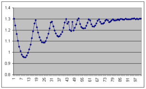
The following graph is a raw data example with \( 20 ms \) between samples. | The following graph is a raw data example with \( 20 ms \) between samples. | ||
| Line 33: | Line 33: | ||
[[File:Gravidade-graf1.png|thumb| Raw data of a launch]] | [[File:Gravidade-graf1.png|thumb| Raw data of a launch]] | ||
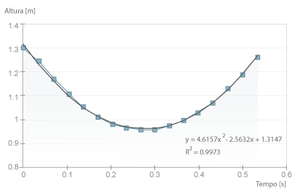
| − | This next graph, with the corrected time, | + | This next graph, with the corrected time and numerical fitted curve, gives the final value \( 9,2 ms^{-2} \) for g. |
[[File:Gravidade-graf2.png|thumb|Fit using the law for the uniform motion applied to one bounce]] | [[File:Gravidade-graf2.png|thumb|Fit using the law for the uniform motion applied to one bounce]] | ||
| − | =Advanced Protocol= | + | =Advanced Protocol I= |
| − | Since the ping-pong ball has very low mass, the air resistance will be significant after the ball reaches a certain speed. This way, if we fit the \( x = v_0 t + \frac{1}{2} g t^2 \) to the data right as the motion starts (\(v_0 \simeq 0\)), we can obtain a numerical value for g that is closer to reality. It is interesting to study on how | + | Since the ping-pong ball has very low mass, the air resistance will be significant after the ball reaches a certain speed. This way, if we fit the \( x = v_0 t + \frac{1}{2} g t^2 \) to the data right as the motion starts (\(v_0 \simeq 0\)), we can obtain a numerical value for <i>g</i> that is closer to reality. It is interesting to study on how <i>g</i> changes with speed and observe it's deviation from the expected value \( 9.8 m/s^{-2} \). It can be observed that for smaller trajectories (when the ball bounces), the numerical results are better, or, likewise, in regions where the speed is lower (when the ball reaches a maximum in height). |
By considering air friction, the fitting of a more adequate function will result in the value found for \( g \) being more precise and will allow the determination of the air friction constant alpha (\( \alpha \)). If we consider friction to be dependant of \( v^2 \) and applying a force opposite to the movement, we can consider the differential equation: | By considering air friction, the fitting of a more adequate function will result in the value found for \( g \) being more precise and will allow the determination of the air friction constant alpha (\( \alpha \)). If we consider friction to be dependant of \( v^2 \) and applying a force opposite to the movement, we can consider the differential equation: | ||
| Line 46: | Line 46: | ||
mg - \alpha v^2 = ma | mg - \alpha v^2 = ma | ||
\] . | \] . | ||
| + | |||
| + | =Advanced Protocol II= | ||
| + | The restitution coefficient can be inferrend from consecutive leaps. It can serve to determine the energy loss in every ball collision and to study its behaviour. | ||
Revision as of 20:38, 2 November 2012
Contents
Description of the Experiment
This experiment allows to determine the standard gravity acceleration, g .
Ligações
- Video: rtsp://elabmc.ist.utl.pt:554/g.sdp
- Laboratório: Básico em e-lab.ist.eu
- Sala de controlo: g
- Nivel: ***
Experimental Apparatus
This apparatus consist in a projectile launcher (with an electromagnet) that vertically ejects a ping-pong ball from the base.
The ping-pong ball is launched with a kinetic energy from the base selected by the user (energy applied to the electromagnet) and executes the typicall parabola trajectory, falling subsequently on the base. The height (vertical coordinate) is measured and recorded with an ultrasound sonar, strategically placed above the experiment, measuring the distance between itself and the ball. With the resulting data it is possible to determine g. The ball is sometimes launched with a small horizontal component, but this does not affect measurements (why?).
Since the height is measured by ultrasounds, the actual time between samples varies from the one provided by the user: the closer the ball is to the sensor (i.e., higher), the shorter the time between samples is. This can be negleted unless a precise fitting is requested.
Protocol
The user must define the following parameters: launch energy, time between samples and number of samples.
The standard gravity, g, can be established in various ways. The simplest is to fit the mathematical law for the ball's motion, \( x = x_0 + v_0 t + \frac{1}{2}gt^2 \), to the experimental data by choosing three points from the space-time graph and solving the system of equations.
The following graph is a raw data example with \( 20 ms \) between samples.
This next graph, with the corrected time and numerical fitted curve, gives the final value \( 9,2 ms^{-2} \) for g.
Advanced Protocol I
Since the ping-pong ball has very low mass, the air resistance will be significant after the ball reaches a certain speed. This way, if we fit the \( x = v_0 t + \frac{1}{2} g t^2 \) to the data right as the motion starts (\(v_0 \simeq 0\)), we can obtain a numerical value for g that is closer to reality. It is interesting to study on how g changes with speed and observe it's deviation from the expected value \( 9.8 m/s^{-2} \). It can be observed that for smaller trajectories (when the ball bounces), the numerical results are better, or, likewise, in regions where the speed is lower (when the ball reaches a maximum in height).
By considering air friction, the fitting of a more adequate function will result in the value found for \( g \) being more precise and will allow the determination of the air friction constant alpha (\( \alpha \)). If we consider friction to be dependant of \( v^2 \) and applying a force opposite to the movement, we can consider the differential equation:
\[ mg - \alpha v^2 = ma \] .
Advanced Protocol II
The restitution coefficient can be inferrend from consecutive leaps. It can serve to determine the energy loss in every ball collision and to study its behaviour.


