Difference between revisions of "Dice Statistics"
m (Text replacement - "\[" to "<math>") |
m (Text replacement - "\]" to "</math>") |
||
| Line 99: | Line 99: | ||
<math> | <math> | ||
p(x) = y_0 + A e ^{- \frac{(x- \mu)^2}{\sigma ^2}} | p(x) = y_0 + A e ^{- \frac{(x- \mu)^2}{\sigma ^2}} | ||
| − | + | </math> | |
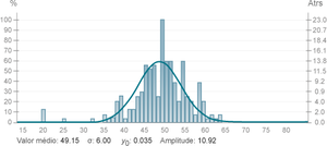
[[File:EstatDados-grafico.png|thumb|Figure 5: Example distribution]] | [[File:EstatDados-grafico.png|thumb|Figure 5: Example distribution]] | ||
| Line 111: | Line 111: | ||
<math> | <math> | ||
\bar{\mu} = \frac{6N+N}{2} | \bar{\mu} = \frac{6N+N}{2} | ||
| − | + | </math> | |
| Line 136: | Line 136: | ||
<math> | <math> | ||
t = \sqrt{\frac{A- 2 A cos (2 \pi f t)}{g}} | t = \sqrt{\frac{A- 2 A cos (2 \pi f t)}{g}} | ||
| − | + | </math> | |
So solve this equation, we have to use a computational method which, having been given an inicial value for t, will evaluate the root and then use the value it finds for t. This process is repeated until t is stationary. Obviouslly, we have to have the values for amplitude, frequency and acceleration. For the first we use 3mm, beteween 1 and 500Hz for the second and 9,81 \(ms^{-2}\) for the last. | So solve this equation, we have to use a computational method which, having been given an inicial value for t, will evaluate the root and then use the value it finds for t. This process is repeated until t is stationary. Obviouslly, we have to have the values for amplitude, frequency and acceleration. For the first we use 3mm, beteween 1 and 500Hz for the second and 9,81 \(ms^{-2}\) for the last. | ||
Revision as of 20:40, 24 May 2015
Contents
Description
This experiment consists of an apparatus that automatically shuffles a set of six-sided dice. To count the spots, it acquires and processes an image recognition pattern from the top side of each dice.
By recording the number of times each side appears, you can study the law of probability and develop a statistical study of random phenomena. Using the images produced by this experiment, you can also develop your own algorithms using them in the study of computer recognition software.
Links
- Video: [unavailable]
- Laboratory: Básico em e-lab.ist.eu[1]
- Control room: Aleatorio
- Grade: ***
<swf height="320" width="320">http://www.elab.tecnico.ulisboa.pt/anexos/descricoes-flash/EstatisticaDados.swf</swf>
Experimental Apparatus
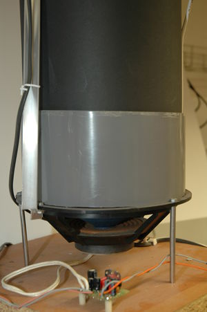
In this experiment there is a loudspeaker positioned horizontally with a platform on top of the cone made of k-line (structured light cardboard with polyurethane), where fourteen dice are spread. Above it, at 300mm from the platform, there is a video camera equipped with a white high brightness LED to illuminate it.
The release (i.e. shuffling) of the dice is achieved through the speaker's stimulus with a sound wave, which makes the platform vibrate with the same frequency of the wave.
This platform has a wall that prevents the dice from leaving the platform (and the web-cam field of view). The wall is quite high to block the entry of light from the outside of the lighting system.
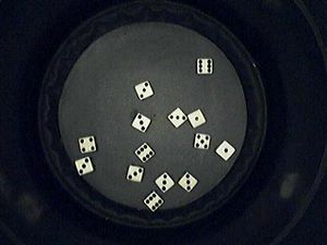
With this apparatus, pictures are obtained as we can see in figure 2.
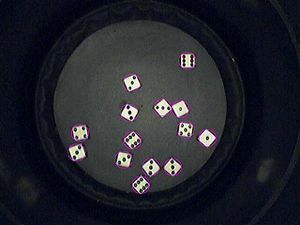
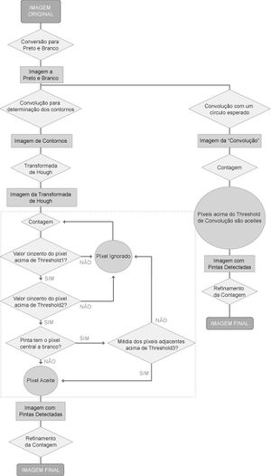
The image processing is made according to the flowchart below and the result of this process leads to an image like the one in picture 3.
Protocol
The experience execution protocol is simple because it consists in stimulating the platform conveniently, so that it can scramble the dice. The main features of the configurator control room are described below for a better understanding.
User Manual
The user can change the parameters of the image recognition process.
- Black&White Threshold: the value, in grayscale, above which the pixels are considered white.
- Hough Transform
- Threshold1: value above which a pixel from the Hough Transform image is taken to post processing.
- Threshold2: averages the pixels near the one that passed the previous test and, if that value is above Threshold2, this pixel is taken to post processing.
- Threshold3: in theory, any pixel in a white zone is ignored but, if the average (calculated in the previous test) is above Threshold3, the pixel is NOT ignored. This is used because some of the dice have white spots inside the black marks.
- Convolution Threshold: the value above which a pixel from the convolution image is taken to post processing.
- Dice specifications:
- Mark radius: the expected radius, given in pixels, of the marks (note that this algorithm expects the marks to be circular).
- Dice width: the maximum distance, in pixels, between marks. For example, in the 6-side of the dice, this value would be diagonal distance from one corner to the other.
- Expected number of dice: the number of dice in the experiment. If the algorithm finds more "dice" (i.e. sets of marks) than expected, and some of those sets are not considered "compatible" with dice, then these sets are eliminated (Note: The algorithm compares the relative position and distance between marks to create a set. These sets are then compared to what is expected in a dice; if the comparison is positive, the set is marked as "compatible", if not, some marks are switched or eliminated until a "compatible" set is achieved).
Dice shuffling
The dice are released (shuffled) by the oscillating movement of the platform where they are located. The user can select the starting and the ending frequencies of the sound wave that will be transmitted to the platform. This sound wave is synthesized on demand, there are no pre-recorded sound files.
The frequency can be chosen between 20Hz and 150Hz. Bellow 20Hz there is no response from the hardware to vibrate the platform; above 150Hz, the inertia "forces" a low amplitude motion, so the dice don't move.
The user can also choose the duration of the sound wave from 1.5 to 10 seconds. The lower value is enough to shuffle some of the dice at lower frequency but it will ultimately result in a small randomization. The upper limit allows very high randomization and is not even necessary in some cases.
Images
The user chooses how many frames should be analysed by choosing the number of samples between 1 and 20.
One sample can be used to check how the recognition software works (what are the steps and how long they take). With 20 samples the results start to show a distribution that evolves towards the Gaussian distribution (even though, in theory, this only happens after 30 samples, minimum).
Video
The user can choose whether to watch or not to watch the shuffling process video.
This video is composed of a series of .jpg pictures, which means that it is not an actual video, and the rate of display can change substantially with the connection quality.
Since the video feed has a high demand on the internet connection, the user is advised to use it only once, as its purpose is merely to satisfy curiosity.
Advanced Protocol
After a number of samples a graph can be constructed with the number of times each number is recorded in each bin and a Gaussian distribution can be fitted:
[math] p(x) = y_0 + A e ^{- \frac{(x- \mu)^2}{\sigma ^2}} [/math]
Since there are 14 dice, the expected mean value is 49 (why?), which is confirmed by the build-up of values fitting.
The best way to conduct this study is to merge the results of several users and see if the fit is improved by an increasing number of samples.
The expected value for the average of N 6-sided dice is:
[math] \bar{\mu} = \frac{6N+N}{2} [/math]
What is the best frequency to randomize the dice?
We assume:
- A die that starts at rest will follow the platform's upward motion;
- The die will only move away from the platform when the latter starts moving down, i.e. the die is in free fall with no initial vertical velocity;
- The bump between die and platform is non-elastic, i.e. it will move with the platform until it returns to the highest position.
So, if we consider the motion that starts when the die and the platform are separated, we can write the following expressions for each dice and the polatform:
Die: \( y(t) = \frac{A}{2} - \frac{g ^2}{2} \)
Platform: \( y'(t) = A cos(2 \pi f t) \)
where A is the platform's motions's amplitude, g is the standard gravity, f is the platform's vibration frequency and t is the time since the die separated from the platform.
Equalizing and solving for t, we get:
[math] t = \sqrt{\frac{A- 2 A cos (2 \pi f t)}{g}} [/math]
So solve this equation, we have to use a computational method which, having been given an inicial value for t, will evaluate the root and then use the value it finds for t. This process is repeated until t is stationary. Obviouslly, we have to have the values for amplitude, frequency and acceleration. For the first we use 3mm, beteween 1 and 500Hz for the second and 9,81 \(ms^{-2}\) for the last.
The t value for the first iteration is 1/4 f, so we get zero for the cosine inside the root and the final result is a real value.
In the following table we can see frequencies and the values for which t converged, as well as the resulting sin and cos:
| f (Hz) | t (milisec.) | cos(2p f t ) | - sin(2p f t ) |
|---|---|---|---|
| 14 | 27.91 | -0.7732 | -0.6341 |
| 15 | 29.70 | -0.9418 | -0.3362 |
| 16 | 30.24 | -0.9948 | -0.1017 |
| 17 | 30.25 | -0.9960 | 0.0893 |
| 18 | 29.98 | -0.9692 | 0.2462 |
| 19 | 29.54 | -0.9268 | 0.3756 |
| 20 | 29.01 | -0.8758 | 0.4827 |
| 21 | 28.42 | -0.8206 | 0.5715 |
| 49 | 30.21 | -0.9924 | 0.1227 |
| 50 | 30.26 | -0.9968 | 0.0805 |
| 51 | 30.06 | -0.9781 | 0.2083 |
| 83 | 30.26 | -0.9973 | 0.0736 |
| 116 | 30.27 | -0.9977 | 0.0680 |
| 149 | 30.27 | -0.9980 | 0.0632 |
| 182 | 30.27 | -0.9983 | 0.0591 |
| 215 | 30.27 | -0.9985 | 0.0554 |
| 248 | 30.28 | -0.9986 | 0.0521 |
| 281 | 30.28 | -0.9988 | 0.0491 |
Trajectories have a common point near the platform's motions's minimum (cos(2pf t ) >> -1), when it is already going up (-sin(2p f t ) >0).
